Bitslicing with Karnaugh maps
Data Orthogonalization for Cryptography
Bitslicing, in cryptography, is the technique of converting arbitrary functions into logic circuits, thereby enabling fast, constant-time implementations of cryptographic algorithms immune to cache and timing-related side channel attacks.
My last post Bitslicing, An Introduction showed how to convert an S-box function into truth tables, then into a tree of multiplexers, and finally how to find the lowest possible gate count through manual optimization.
Today’s post will focus on a simpler and faster method. Karnaugh maps help simplifying Boolean algebra expressions by taking advantage of humans’ pattern-recognition capability. In short, we’ll bitslice an S-box using K-maps.
Part 1: Bitslicing, An Introduction
Part 2: Bitslicing with Karnaugh maps
Part 3: Bitslicing with Quine-McCluskey
A tiny S-box
Here again is the 3-to-2-bit S-box function from the previous post.
uint8_t SBOX[] = { 1, 0, 3, 1, 2, 2, 3, 0 };
An AES-inspired S-box that interprets three input bits as a polynomial in GF(23) and computes its inverse mod P(x) = x3 + x2 + 1, with 0-1 := 0. The result plus (x2 + 1) is converted back into bits and the MSB is dropped.
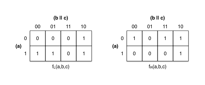
This S-box can be represented as a function of three Boolean variables, where f(0,0,0) = 0b01, f(0,0,1) = 0b00, f(0,1,0) = 0b11, etc. Each output bit can be represented by its own Boolean function where fL(0,0,0) = 0 and fR(0,0,0) = 1, fL(0,0,1) = 0 and fR(0,0,1) = 0, …
A truth table per output bit
Each output bit has its own Boolean function, and therefore also its own thruth table. Here are the truth tables for the Boolean functions fL(a,b,c) and fR(a,b,c):
| abc | out |
|---|---|
| 000 | 01 |
| 001 | 00 |
| 010 | 11 |
| 011 | 01 |
| 100 | 10 |
| 101 | 10 |
| 110 | 11 |
| 111 | 00 |
| abc | out |
|---|---|
| 000 | 0 |
| 001 | 0 |
| 010 | 1 |
| 011 | 0 |
| 100 | 1 |
| 101 | 1 |
| 110 | 1 |
| 111 | 0 |
| abc | out |
|---|---|
| 000 | 1 |
| 001 | 0 |
| 010 | 1 |
| 011 | 1 |
| 100 | 0 |
| 101 | 0 |
| 110 | 1 |
| 111 | 0 |
Whereas previously at this point we built a tree of multiplexers out of each truth table, we’ll now build a Karnaugh map (K-map) per output bit.
Karnaugh Maps
The values of fL(a,b,c) and fR(a,b,c) are transferred onto a two-dimensional grid with the cells ordered in Gray code. Each cell position represents one possible combination of input bits, while each cell value represents the value of the output bit.
The row and column indices (a) and (b || c) are ordered in Gray code rather
than binary numerical order to ensure only a single variable changes between
each pair of adjacent cells. Otherwise, products of predicates
(a & b, a & c, …) would scatter.
These products are what you want to find to get a minimum length representation
of the truth function. If the output bit is the same at two adjacent cells,
then it’s independent of one of the two input variables, because
(a & ~b) | (a & b) = a.
Spotting patterns
The heart of simplifying Boolean expressions via K-maps is finding groups of
adjacent cells with value 1. The rules are as follows:
- Groups are rectangles of 2n cells with value
1. - Groups may not include cells with value
0. - Each cell with value
1must be in at least one group. - Groups may be horizontal or vertical, not diagonal.
- Each group should be as large as possible.
- There should be as few groups as possible.
- Groups may overlap.
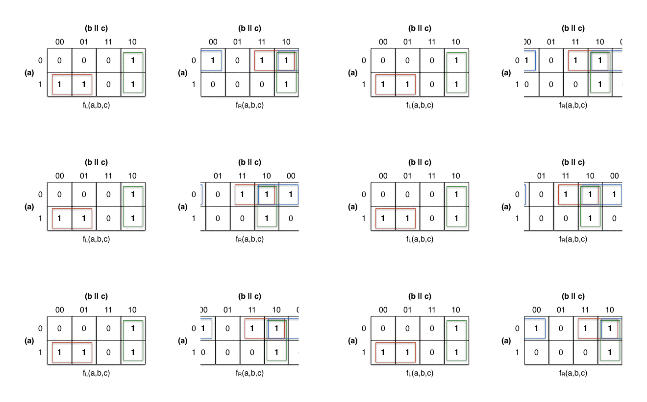
First, we mark all cells with value 1. We then form a red
group for the two horizontal groups of size 21. The two vertical groups are
marked with green, also of size 21.
On fR’s K-map on the right, the red
and green group overlap. As per the rules
above, that’s perfectly fine. The cell at abc=110 can’t be without a group
and we’re instructed to form the largest groups possible, so they overlap.
But wait, you say, what’s going on with the blue rectangle on the right?
Wrapping around
A somewhat unexpected property of K-maps is that they’re not really grids, but actually toruses. In plain English: they wrap around the top, bottom, and the sides.
Look at this neat animation on Wikipedia
that demonstrates how a rectangle can turn into a donuttorus. Adjacent
thus has a special definition here: cells on the very right touch those on the
far left, as do those at the very top and bottom.
Another way to understand this property is to imagine that the columns don’t
start at 00 but rather at 01, and so we rotate the whole K-map by one to
the left. Then the rectangles wouldn’t need to wrap around and they would all
fit on the grid nicely.
Now that all cells with a 1 have been assigned to as few groups as possible,
let’s get our hands dirty and write some code.
A bitsliced SBOX() function
K-maps are read groupwise: we look at each cell’s position and focus on the input values that do not change throughout the group. Values that do change are ignored.
One function for fL(a,b,c) ...
The red group covers the cells at position
100 and 101. The values a=1 and b=0 are constant, they will be included
into the group’s term. The value of c changes and is therefore irrelevant.
The term is (a & ~b).
The green group covers the cells at 010
and 110. We ignore a, and include b=1 and c=0. The term is (b & ~c).
SBOXL() is the disjunction of the group terms we collected from the K-map. It
lists all possible combinations of input values that lead to output value 1.
uint8_t SBOXL(uint8_t a, uint8_t b, uint8_t c) {
  return (a & ~b) | (b & ~c);
}
... and another one for fR(a,b,c)
The red group covers the cells at 011
and 010. The term is (~a & b).
The green group covers the cells at 010
and 110. The term is (b & ~c).
The blue group covers the cells at 000
and 010. The term is (~a & ~c).
uint8_t SBOXR(uint8_t a, uint8_t b, uint8_t c) {
  return (~a & b) | (b & ~c) | (~a & ~c);
}
Great, that’s all we need! Now we can merge those two functions and compare that to the result of the previous post.
Putting it all together
The first three variables ensure that we negate inputs only once. t0 replaces
the common subexpression b & nc. Any optimizing compiler would do the same.
void SBOX(uint8_t a, uint8_t b, uint8_t c, uint8_t* l, uint8_t* r) {
  uint8_t na = ~a;
  uint8_t nb = ~b;
  uint8_t nc = ~c;

  uint8_t t0 = b & nc;

  *l = (a & nb) | t0;
  *r = (na & b) | (na & nc) | t0;
}
Ten gates. That’s one more than the manually optimized version from the last post. What’s missing? Turns out that K-maps sometimes don’t yield the minimal form and we have to simplify further by taking out common factors.
The conjunctions in the term (na & b) | (na & nc) have the common factor na
and, due to the Distributivity Law, can be rewritten as na & (b | nc). That
removes one of the AND gates and leaves two.
void SBOX(uint8_t a, uint8_t b, uint8_t c, uint8_t* l, uint8_t* r) {
  uint8_t na = ~a;
  uint8_t nb = ~b;
  uint8_t nc = ~c;

  uint8_t t0 = b & nc;
  uint8_t t1 = b | nc;

  *l = (a & nb) | t0;
  *r = (na & t1) | t0;
}
Nine gates. That’s exactly what we achieved by tedious artisanal optimization.
More than four inputs
K-maps are neat and trivial to use once you’ve worked through an example yourself. They yield minimal circuits fast, compared to manual optimization where the effort grows exponentially with the number of terms.
There is one downside though, and it’s that the original variant of a K-map can’t be used with more than four input variables. There are variants that do work with more than four variables but they actually make it harder to spot groups visually.
The Quine–McCluskey algorithm is functionally identical to K-maps but can handle an arbitrary number of input variables in its original variant – although the running time grows exponentially with the number of variables. Not too problematic for us, S-boxes usually don’t have too many inputs anyway…


